Draw Gaussian Distribution
Draw Gaussian Distribution - Also choose to plot the data as an xy graph of points. Web the graph of a gaussian function forms the characteristic bell shape of the gaussian/normal distribution, and has the general form. Web ©2021 matt bognar department of statistics and actuarial science university of iowa The first step is to set up the environment: When plotted on a graph, the data follows a bell shape, with most values clustering around a central region and tapering off as they go further away from the center. We take an extremely deep dive into the normal distribution to explore the parent function that generates normal distributions, and how to modify parameters in the function. Normal distributions are also called gaussian distributions or bell curves because of their shape. The trunk diameter of a certain variety of pine tree is normally distributed with a mean of μ = 150 cm and a standard deviation of σ = 30 cm. Graph functions, plot points, visualize algebraic equations, add sliders, animate graphs, and more. Lisa yan and jerry cain, cs109, 2020 quick slide reference 2 3 normal rv 10a_normal 15 normal rv:
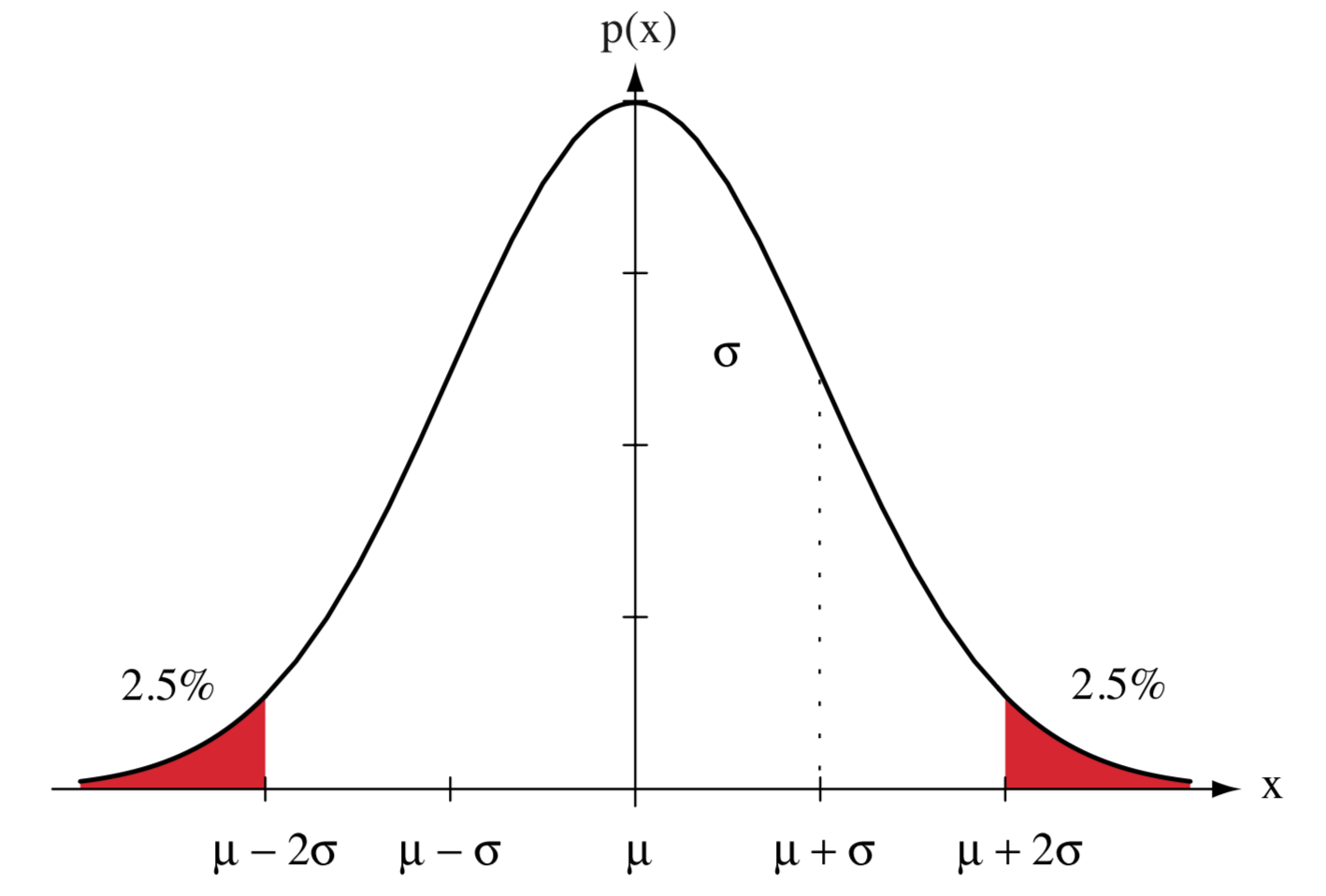
Graph functions, plot points, visualize algebraic equations, add sliders, animate graphs, and more. Normal distributions are also called gaussian distributions or bell curves because of their shape. Julia> using random, distributions julia> random.seed!(123) # setting the seed. The first step is to set up the environment: Web (gaussian) distribution lisa yan and jerry cain october 5, 2020 1. Web maths physics statistics probability graph. The green shaded area represents the probability of an event with mean μ, standard deviation σ occuring between x1 and x2, while the gray shaded area is the normalized case, where. The general form of its probability density function is The gaussian distribution, (also known as the normal distribution) is a probability distribution. Web in a normal distribution, data is symmetrically distributed with no skew.
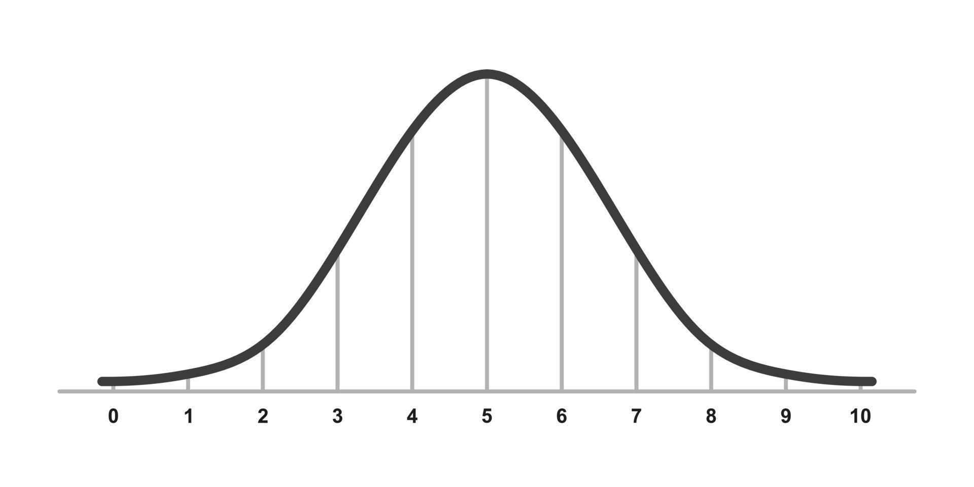
Web draw random samples from a normal (gaussian) distribution. The probability density function of the normal distribution, first derived by de moivre and 200 years later by both gauss and laplace independently , is often called the bell curve because of its characteristic shape (see the example below). In statistics, a bell curve (also known as a standard normal distribution or gaussian curve) is a symmetrical graph that illustrates the tendency of data to cluster around a center value, or mean, in a given dataset. When plotted on a graph, the data follows a bell shape, with most values clustering around a central region and tapering off as they go further away from the center. Web in this tutorial, you’ll learn how to use the numpy random.normal function to create normal (or gaussian) distributions. Such a distribution is specified by. Web ©2021 matt bognar department of statistics and actuarial science university of iowa The mean of 150 cm goes in the middle. Web in a normal distribution, data is symmetrically distributed with no skew. The trunk diameter of a certain variety of pine tree is normally distributed with a mean of μ = 150 cm and a standard deviation of σ = 30 cm.

Gaussian Distribution Explained Visually Intuitive Tutorials
In statistics, a bell curve (also known as a standard normal distribution or gaussian curve) is a symmetrical graph that illustrates the tendency of data to cluster around a center value, or mean, in a given dataset. The mean of 150 cm goes in the middle. Where a, b, and c are real constants, and c ≠ 0. When plotted.
The Gaussian Distribution Video Tutorial & Practice Channels for Pearson+
Web draw random samples from a multivariate normal distribution. In a gaussian distribution, the parameters a, b, and c are based on the mean (μ) and standard deviation (σ). Web import numpy as np import matplotlib.pyplot as plt mean = 0; Sketch a normal curve that describes this distribution. In statistics, a bell curve (also known as a standard normal.
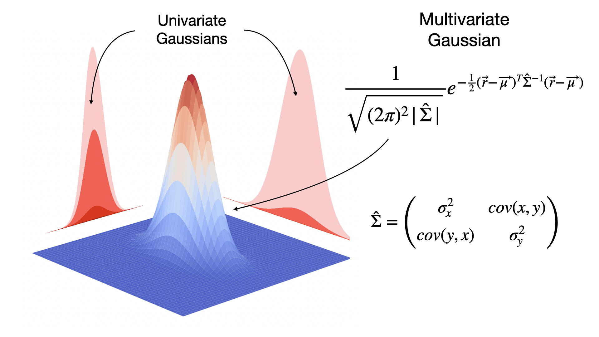
Visualizing a multivariate Gaussian
The first step is to set up the environment: In [1]:= out [1]= in [2]:= out [2]= in [3]:= out [3]= Properties 10b_normal_props 21 normal rv: The gaussian distribution, (also known as the normal distribution) is a probability distribution. 2.go to the new graph.
Gauss distribution. Standard normal distribution. Gaussian bell graph
In [1]:= out [1]= in [2]:= out [2]= in [3]:= out [3]= Computing probability 10c_normal_prob 30 exercises live. Web in a normal distribution, data is symmetrically distributed with no skew. The general form of its probability density function is Lisa yan and jerry cain, cs109, 2020 quick slide reference 2 3 normal rv 10a_normal 15 normal rv:

Gaussian Distribution Explained Visually Intuitive Tutorials
Normal distributions are also called gaussian distributions or bell curves because of their shape. Sketch a normal curve that describes this distribution. Basic examples (4) probability density function: Properties 10b_normal_props 21 normal rv: In [1]:= out [1]= in [2]:= out [2]= in [3]:= out [3]=

1 The Gaussian distribution labeled with the mean µ y , the standard
In [1]:= out [1]= in [2]:= out [2]= in [3]:= out [3]= In a gaussian distribution, the parameters a, b, and c are based on the mean (μ) and standard deviation (σ). Normaldistribution [] represents a normal distribution with zero mean and unit standard deviation. Web maths physics statistics probability graph. 3.click analyze, choose nonlinear regression, and choose the one.
Normal Distribution Gaussian Distribution Bell Curve Normal Curve
Also choose to plot the data as an xy graph of points. Web in this tutorial, you’ll learn how to use the numpy random.normal function to create normal (or gaussian) distributions. The gaussian distribution, (also known as the normal distribution) is a probability distribution. The starting and end points of the region of interest ( x1 and x2, the green.
The Gaussian Distribution The Beard Sage
Lisa yan and jerry cain, cs109, 2020 quick slide reference 2 3 normal rv 10a_normal 15 normal rv: Web drawing a normal distribution example. Web maths physics statistics probability graph. Web (gaussian) distribution lisa yan and jerry cain october 5, 2020 1. Web import numpy as np import matplotlib.pyplot as plt mean = 0;
Gauss distribution. Standard normal distribution. Gaussian bell graph
The normal distributions occurs often in. Web maths physics statistics probability graph. The green shaded area represents the probability of an event with mean μ, standard deviation σ occuring between x1 and x2, while the gray shaded area is the normalized case, where. Computing probability 10c_normal_prob 30 exercises live. Sketch a normal curve that describes this distribution.
Gauss distribution. Standard normal distribution. Gaussian bell graph
Web the graph of a gaussian function forms the characteristic bell shape of the gaussian/normal distribution, and has the general form. Also choose to plot the data as an xy graph of points. Such a distribution is specified by. Web represents a normal (gaussian) distribution with mean μ and standard deviation σ. The starting and end points of the region.
Web ©2021 Matt Bognar Department Of Statistics And Actuarial Science University Of Iowa
Properties 10b_normal_props 21 normal rv: Web import numpy as np import matplotlib.pyplot as plt mean = 0; The green shaded area represents the probability of an event with mean μ, standard deviation σ occuring between x1 and x2, while the gray shaded area is the normalized case, where. The starting and end points of the region of interest ( x1 and x2, the green dots).
We Take An Extremely Deep Dive Into The Normal Distribution To Explore The Parent Function That Generates Normal Distributions, And How To Modify Parameters In The Function.
Web draw random samples from a normal (gaussian) distribution. Lisa yan and jerry cain, cs109, 2020 quick slide reference 2 3 normal rv 10a_normal 15 normal rv: The functions provides you with tools that allow you create distributions with specific means and standard distributions. Where a, b, and c are real constants, and c ≠ 0.
Web The Graph Of A Gaussian Function Forms The Characteristic Bell Shape Of The Gaussian/Normal Distribution, And Has The General Form.
Normaldistribution [] represents a normal distribution with zero mean and unit standard deviation. Normal distributions are also called gaussian distributions or bell curves because of their shape. Web in this tutorial, you’ll learn how to use the numpy random.normal function to create normal (or gaussian) distributions. Web explore math with our beautiful, free online graphing calculator.
Such A Distribution Is Specified By.
In [1]:= out [1]= in [2]:= out [2]= in [3]:= out [3]= In a gaussian distribution, the parameters a, b, and c are based on the mean (μ) and standard deviation (σ). In statistics, a bell curve (also known as a standard normal distribution or gaussian curve) is a symmetrical graph that illustrates the tendency of data to cluster around a center value, or mean, in a given dataset. Julia> using random, distributions julia> random.seed!(123) # setting the seed.