How To Draw Pareto In Excel
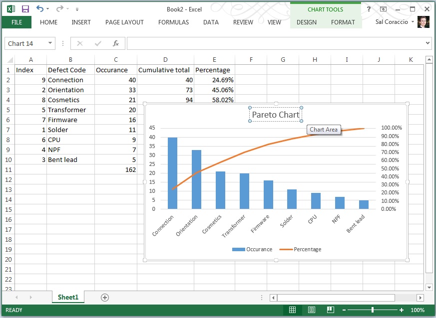
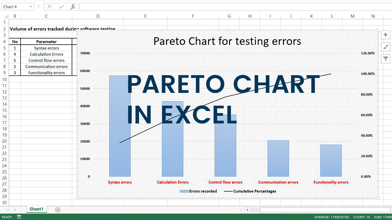
How To Draw Pareto In Excel - This inserts a column chart with 2 series of data (# of complaints and the cumulative percentage). From the insert tab, select ‘recommended charts.’. Select both columns of data. So if my mean calculated out at 16 excel would show that as an exceptional first. From this list, select the chart type ‘histogram’. You can do this by following these steps: Under histogram, there are further two options. How to create a pareto chart in excel 2007, 2010, and 2013. Remember, a pareto chart is a sorted histogram chart. A cumulative percent line is.
Web join the free course 💥 top 30 excel productivity tips: In the sort warning dialog box, select sort. See how calculations can be used to add columns to the existing data in excel table. Go to insert tab > charts group > recommended charts. From the ribbon, click the insert tab. Web the steps to create and insert a pareto chart in excel for the above table are: Web click insert > insert statistic chart, and then under histogram, pick pareto. To do so, we will select the sales column >> go to the home. Under histogram, there are further two options. Set up your data as shown below.
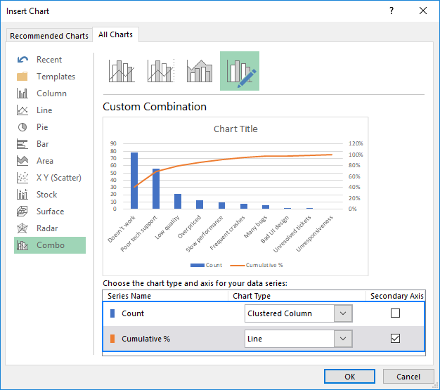
Use multiple pivot tables and pivot charts to create our first dashboard. Set up your data as shown below. In the sort warning dialog box, select sort. From the insert chart dialog box, go to the tab ‘all charts’. Web let’s go through the steps below to analyze sales data using a pareto chart. Go to insert tab > charts group > recommended charts. Then, enter a value of 100 manually and close the “format axis” window. First, click on a cell in the above table to select the entire table. Select any data from the pivot table and click as follows: Web learn about excel tables and what is their advantage over regular ranges.

Pareto chart in Excel how to create it
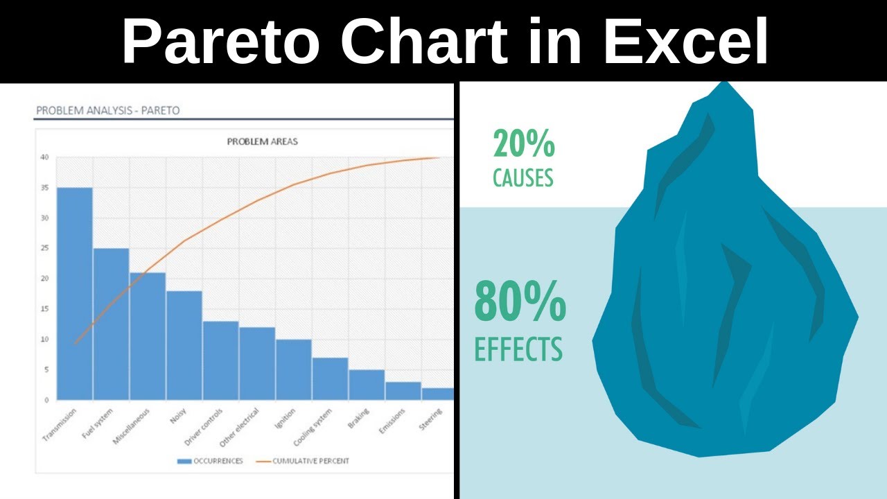
This inserts a column chart with 2 series of data (# of complaints and the cumulative percentage). Web learn how to create a pareto chart, based on the pareto principle or 80/20 rule, in microsoft excel 2013. Our pivot table is ready to create a pareto chart now. You'll see your categories as the horizontal axis and your numbers as.
Make Pareto chart in Excel
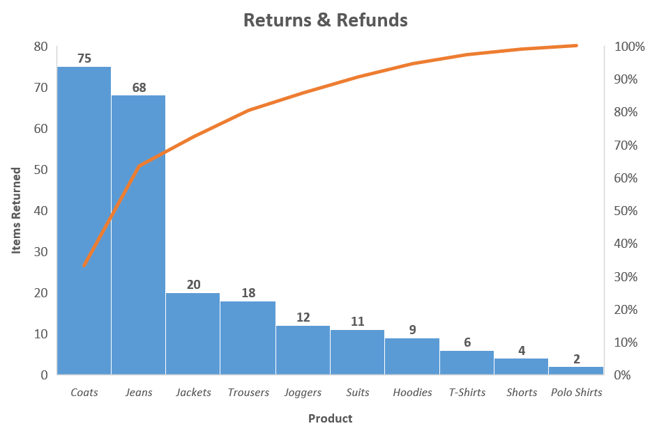
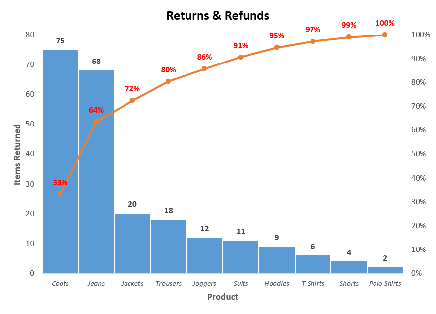
The first one is to create an additional column to translate each of the texts to a numerical value. Excel will create a bar chart with the groups in descending order, calculate the percentages, and include a. Our pivot table is ready to create a pareto chart now. This is a useful lean six sigma or project m. Enter data.
How to use pareto chart in excel 2013 careersbeach
Go back to your onedrive account to find your newly created sheet. Go to insert tab > charts group > recommended charts. The next step is to select a color scheme for your dashboard. Web in this video, i am going to show you how to create a pareto chart in excel.a pareto chart is a type of chart that.
How to Plot Pareto Chart in Excel ( with example), illustration
From the insert tab, select ‘recommended charts.’. You can do this by following these steps: The first step is to enter your data into a worksheet. And just like that, a pareto chart pops into your spreadsheet. Web let’s go through the steps below to analyze sales data using a pareto chart.
How to Create a Pareto Chart in Excel Automate Excel
In the sort warning dialog box, select sort. Under histogram, there are further two options. Web learn about excel tables and what is their advantage over regular ranges. Before you can create a pareto chart in excel, you’ll need to set up your workbook properly. First, click on a cell in the above table to select the entire table.
How to Create Pareto Chart in Microsoft Excel? My Chart Guide
Our pivot table is ready to create a pareto chart now. In the sort warning dialog box, select sort. Join our tutorial to optimize your excel experience with this versatile feature. And then, choose the options insert > insert statistic chart > pareto. Pivottable analyze > tools > pivotchart.
How to Create a Pareto Chart in Excel Automate Excel
Before you can create a pareto chart in excel, you’ll need to set up your workbook properly. From this list, select the chart type ‘histogram’. Enter data and edit your worksheet as desired. And then, choose the options insert > insert statistic chart > pareto. Select the data range, including the column headings.
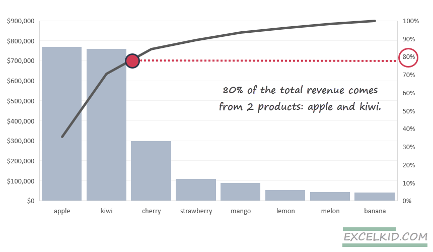
How to create a Pareto chart in Excel Quick Guide Excelkid
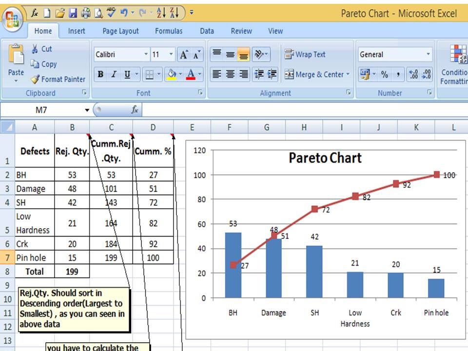
How to create a pareto chart in excel 2016+. Later, select the base field and press ok. Web after you open excel, the first step is to ensure the data analysis toolpak is active. Web click insert > insert statistic chart, and then under histogram, pick pareto. First of all, we have to sort the data in descending order.
Create Pareto Chart In Excel YouTube
Use the design and format tabs to customize the look of your chart. Web here are the steps to create a pareto chart in excel: This is a useful lean six sigma or project m. From the ribbon, click the insert tab. And just like that, a pareto chart pops into your spreadsheet.
How to Create a Pareto Chart in Excel Automate Excel
Web learn how to enhance your microsoft excel spreadsheets with interactive checkboxes/checklists. Use the design and format tabs to customize the look of your chart. The next step is to select a color scheme for your dashboard. Go back to your onedrive account to find your newly created sheet. Enter data and edit your worksheet as desired.
Web Hello, In This Video I Am Going To Show You How An Easy And Fast Way To Make A Perfect Pareto Diagram In Excel.
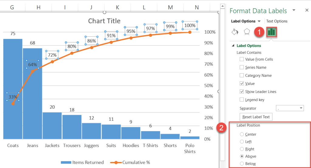
A pareto chart combines a column chart and a line graph. Then, under the “axis” option tab, select “maximum” to set it to be fixed and set the value to 100. This is a useful lean six sigma or project m. And then, choose the options insert > insert statistic chart > pareto.
See How Calculations Can Be Used To Add Columns To The Existing Data In Excel Table.
Pivottable analyze > tools > pivotchart. Under histogram, there are further two options. Use multiple pivot tables and pivot charts to create our first dashboard. Web learn how to create a pareto chart, based on the pareto principle or 80/20 rule, in microsoft excel 2013.
From The Dialog Box That Appears, Select ‘All Charts’ In The Left Pane And ‘Pareto’ In The Right Pane.
Excel will create a bar chart with the groups in descending order, calculate the percentages, and include a. Switch to the all charts tab, select histogram in the left pane, and click on the pareto. Use a table to filter, sort and see totals. This inserts a column chart with 2 series of data (# of complaints and the cumulative percentage).
The First One Is To Create An Additional Column To Translate Each Of The Texts To A Numerical Value.
And just like that, a pareto chart pops into your spreadsheet. Web let’s go through the steps below to analyze sales data using a pareto chart. Create our first pivot table. First of all, we have to sort the data in descending order.